Intro to mapping in R
Preamble
Hello! Here’s an introduction to mapping in R. In this workshop, we will:
- Learn about types of spatial data
- Learn about packages that give us access to open source environmental data in R
- Learn about key operations for manipulating spatial data in R
- Learn about
rgbif, a package for accessing the Global Biodiversity Information Facility (GBIF), a global, open source dataset of species occurrence
I wrote this workshop for IDDO’s R practical session. The intended audience for the workshop was R beginners (if you know the difference between the console and the terminal then you’re not a beginner any more!), but I haven’t provided as much written content as is needed for this to be particularly useful. Either way, I’m popping it here for now and will probably come back to it in future when the need arises.
Download the workshop as an .Rmd and run it for yourself
here.
Resources
Today I’m working from/plagiarising the following useful resources:
- Spatial data with R and
terra(https://rspatial.org/index.html) - Spatial statistics for data science: theory and practice with R (https://www.paulamoraga.com/book-spatial/index.html)
- Introduction to visualising spatial data in R (https://cran.r-project.org/doc/contrib/intro-spatial-rl.pdf)
- A very brief introduction to species distribution modelling in R (https://jcoliver.github.io/learn-r/011-species-distribution-models.html)
- How to (quickly) enrich a map with natural and anthropic details (http://francescobailo.net/2018/08/how-to-quickly-enrich-a-map-with-natural-and-anthropic-details/)
Useful packages
library(raster)  # for bread and butter
library(terra)  # masks lots of the functionality in `raster`
library(sf)  # replaces lots of the functionality in `sp`

library(ggplot2)  # some say this is required to make nice maps in R .. not I!
library(ggmap)  # extends ggplot for maps

library(dplyr)
library(tidyr)
library(tidyverse)
Types of spatial data
There are a couple of different types of data:
- vector data
- points
- lines (and networks)
- polygons
- raster data
All types come with their own things to think about!
See https://rspatial.org/spatial/2-spatialdata.html
(If you would rather see the plot in the Viewer pane, go to RStudio > Preferences > R Markdown and unselect “Show output inline for all R Markdown documents”)
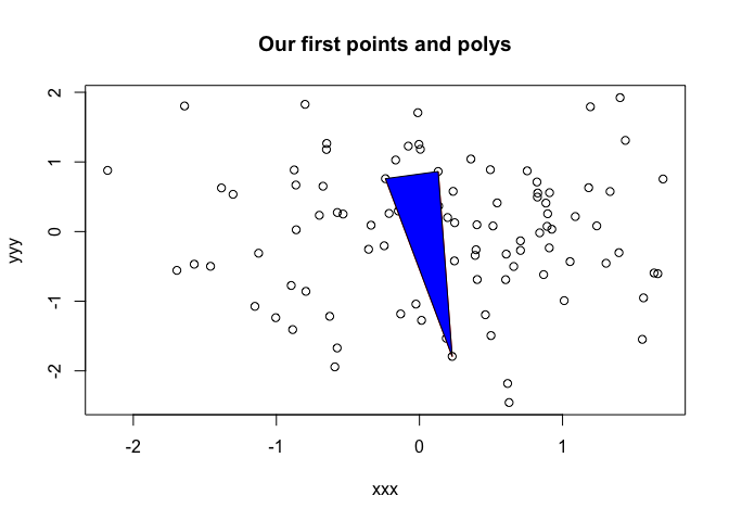
xxx <- rnorm(100)
yyy <- rnorm(100)

plot(xxx, yyy, main="Our first points and polys")

sel <- sample(100, 3)

lines(xxx[sel], yyy[sel], col="red")

polygon(xxx[c(sel, sel[1])], yyy[c(sel, sel[1])], col="blue")
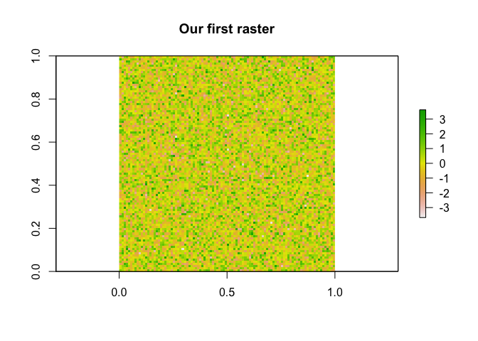
?raster # have a look at some of the arguments here

ras <- rnorm(10000) %>%
  matrix(100, 100) %>%
  raster()

plot(ras, main="Our first raster")
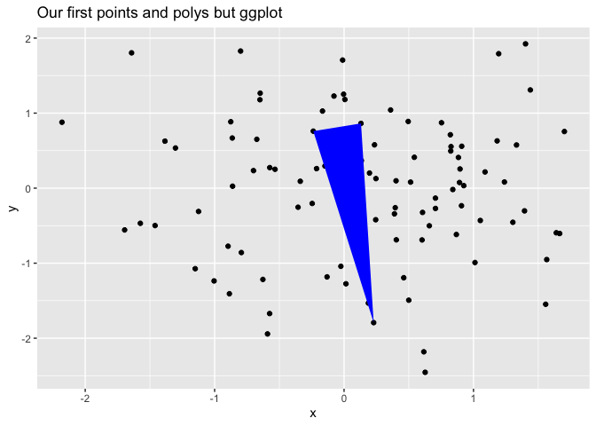
(And here we go in ggplot:)
df = data.frame(x = xxx, y = yyy)

ggplot() +
  geom_point(data = df, aes(x, y)) +
  geom_polygon(data = df[c(sel, sel[1]),], aes(x, y), fill="blue") +
  labs(title = "Our first points and polys but ggplot")
ggplot(rasterToPoints(ras)) + # this is rather silly !!
  geom_raster(aes(x = x, y = y, fill = layer)) +
  scale_fill_viridis_c() +
  labs(title = "Our first raster but ggplot")

Data for case studies
Shapes
Here are some polygons in the wild:
library(geodata)
aus <- gadm("AUS", level = 1, path="~/Desktop/")

aus
##  class       : SpatVector
##  geometry    : polygons
##  dimensions  : 11, 11  (geometries, attributes)
##  extent      : 112.9211, 159.1092, -55.11694, -9.142176  (xmin, xmax, ymin, ymax)
##  coord. ref. : lon/lat WGS 84 (EPSG:4326)
##  names       :   GID_1 GID_0   COUNTRY          NAME_1 VARNAME_1 NL_NAME_1
##  type        :   <chr> <chr>     <chr>           <chr>     <chr>     <chr>
##  values      : AUS.1_1   AUS Australia Ashmore and Ca~        NA        NA
##                AUS.2_1   AUS Australia Australian Cap~        NA        NA
##                AUS.3_1   AUS Australia Coral Sea Isla~        NA        NA
##     TYPE_1 ENGTYPE_1  CC_1 HASC_1  ISO_1
##      <chr>     <chr> <chr>  <chr>  <chr>
##  Territory Territory    12  AU.AS     NA
##  Territory Territory     8  AU.AC AU-ACT
##  Territory Territory    11  AU.CR     NA
Make sure you change the path argument above! Try changing the iso code
to another country! Have a look at the directory where our polygon is
saved: geodata has provided us with an .rds of SpatVectors (from
terra) for Australia. Let’s get these into sf formats and simplify
them down a little …
aus$NAME_1
##  [1] "Ashmore and Cartier Islands"  "Australian Capital Territory"
##  [3] "Coral Sea Islands Territory"  "Jervis Bay Territory"
##  [5] "New South Wales"              "Northern Territory"
##  [7] "Queensland"                   "South Australia"
##  [9] "Tasmania"                     "Victoria"
## [11] "Western Australia"
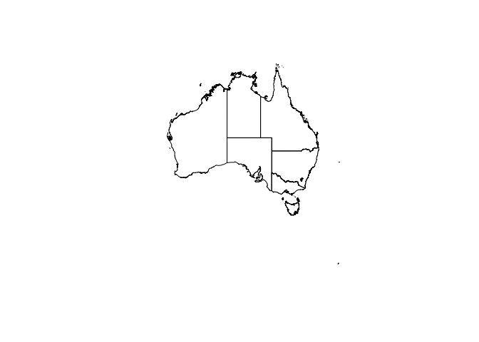
aus <- aus %>%
  st_as_sf()

aus <- aus[c(2,5:11),] # I thought I could do this with a slice()?

plot(st_geometry(st_simplify(aus, dTolerance=1000)))  # dTolerance is in metres !
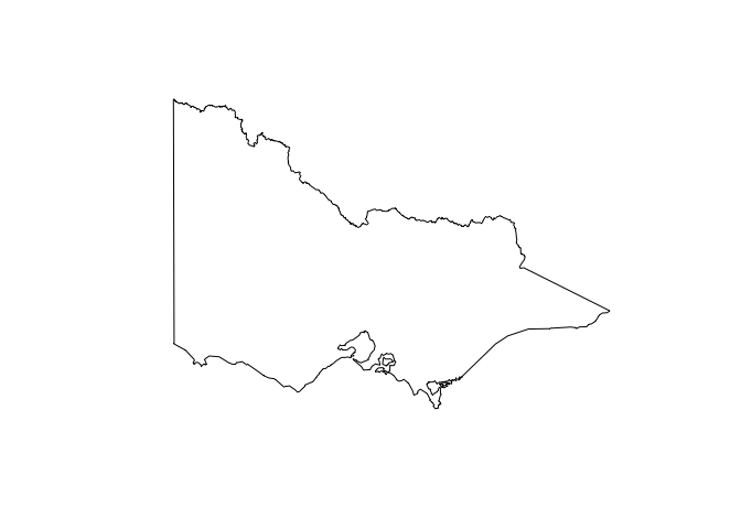
# zoom into Vic for fun
vic <- aus %>%
  filter(NAME_1 == "Victoria") %>%
  st_simplify(dTolerance = 1000)

plot(st_geometry(vic))
Surfaces
Elevation
Let’s meet some raster data in the wild! The elevatr package lets us
access global elevation data.
library(elevatr)
## elevatr v0.99.0 NOTE: Version 0.99.0 of 'elevatr' uses 'sf' and 'terra'.  Use
## of the 'sp', 'raster', and underlying 'rgdal' packages by 'elevatr' is being
## deprecated; however, get_elev_raster continues to return a RasterLayer.  This
## will be dropped in future versions, so please plan accordingly.
vic_elevation <- get_elev_raster(vic, z = 6) # z is zoom ... may need to adjust
## Mosaicing & Projecting

## Note: Elevation units are in meters.
vic_elevation # have a look at all of the information associated with our raster
## class      : RasterLayer
## dimensions : 906, 1129, 1022874  (nrow, ncol, ncell)
## resolution : 0.009960519, 0.009960519  (x, y)
## extent     : 140.625, 151.8704, -40.97639, -31.95216  (xmin, xmax, ymin, ymax)
## crs        : +proj=longlat +datum=WGS84 +no_defs
## source     : file5ea86580a2ff.tif
## names      : file5ea86580a2ff
plot(vic_elevation, main="Elevation in metres")
plot(st_geometry(vic), add = TRUE, border = "blue")
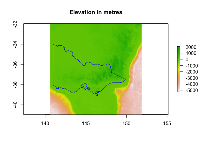
The map we’ve just made is a little hard to read: we can’t tell the difference between ocean pixels and land pixels. To remove ocean pixels, we’ll need to mask and crop our raster.
vic_elevation_masked <- mask(vic_elevation, vic) %>%
  crop(vic) # see what happens without the crop first :)

plot(vic_elevation_masked, main="Elevation in metres")
plot(st_geometry(vic), add=TRUE, border="blue")
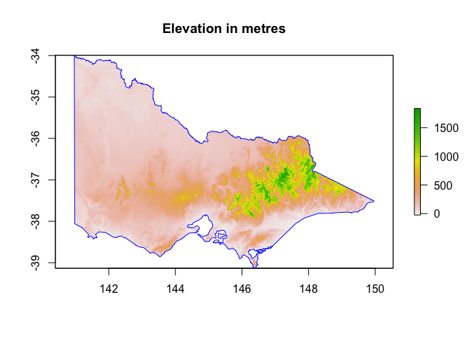
# This picture looks rather different !
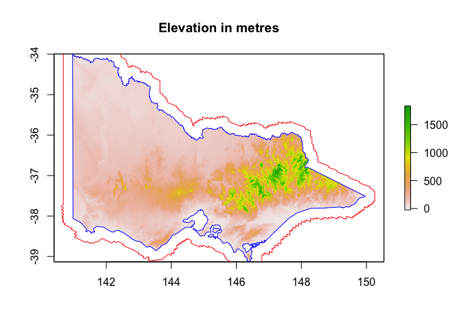
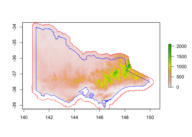
But wait a second! What if I want to be able to see what’s happening in my raster near the land borders? Not to worry! We can buffer and trim!
# First let's have a look at a buffered polygon ...
vic_buffered <- st_buffer(vic, 25000)
plot(vic_elevation_masked, main="Elevation in metres")
plot(st_geometry(vic), add=TRUE, border="blue")
plot(st_geometry(vic_buffered), add=TRUE, border="red")
# Mask elevation raster with all of Australia first (to remove ocean pixels)
vic_elevation_buffered <- mask(vic_elevation, aus) %>%
  mask(vic_buffered) %>% # Then mask with buffered Vic
  trim()

plot(vic_elevation_buffered) # note the fun little hole where the polygons don't quite overlap :)
plot(st_geometry(vic_buffered), add=TRUE, border="red")
plot(st_geometry(vic), add=TRUE, border="blue")
Distance from river / city
library(rnaturalearth)
library(rnaturalearthdata)
##
## Attaching package: 'rnaturalearthdata'

## The following object is masked from 'package:rnaturalearth':
##
##     countries110
rivers <- ne_download(scale =  10, type = 'rivers_lake_centerlines',
                      category = 'physical', returnclass = "sf")
## Reading layer `ne_10m_rivers_lake_centerlines' from data source
##   `/private/var/folders/d3/y1ry00t94rbg0nbfhc8z23p80000gr/T/RtmphBQ8nX/ne_10m_rivers_lake_centerlines.shp'
##   using driver `ESRI Shapefile'
## Simple feature collection with 1473 features and 38 fields
## Geometry type: MULTILINESTRING
## Dimension:     XY
## Bounding box:  xmin: -164.9035 ymin: -52.15775 xmax: 177.5204 ymax: 75.79348
## Geodetic CRS:  WGS 84
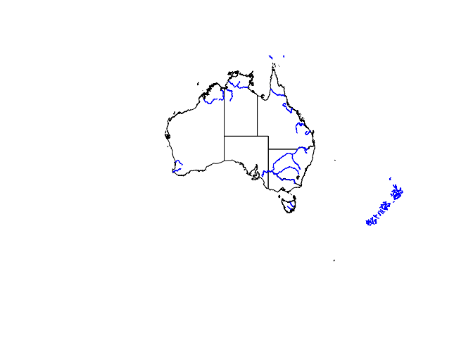
aus_rivers <- rivers %>%
  st_crop(aus)
## Warning: attribute variables are assumed to be spatially constant throughout
## all geometries
plot(st_geometry(st_simplify(aus, dTolerance=1000)))
plot(st_geometry(rivers), col="blue", add=TRUE) # lol I've picked up In Zid
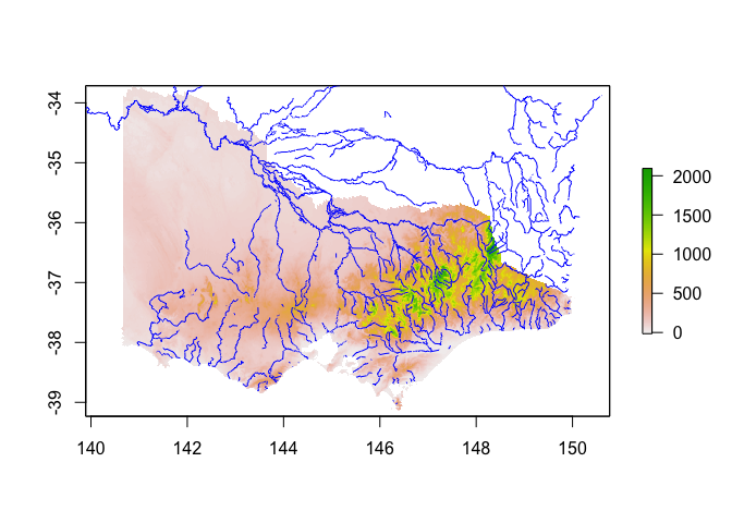
# I would like more rivers !

library(osmdata)
## Data (c) OpenStreetMap contributors, ODbL 1.0. https://www.openstreetmap.org/copyright
osm_rivers <- opq(bbox = st_bbox(vic)) %>%
  add_osm_feature(key = 'waterway', value = 'river') %>%
  osmdata_sf()

osm_rivers <- osm_rivers$osm_lines %>%
  st_simplify(dTolerance = 1000)

osm_rivers <- filter(osm_rivers, !st_is_empty(osm_rivers))

plot(vic_elevation_buffered)
plot(st_geometry(osm_rivers), add=TRUE, col="blue")
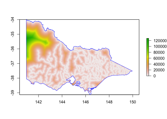
A very handy modelling covariate can be distance from a watercourse -
let’s cheekily do that with terra:
dist_to_rivers <- vic_elevation

rivers <- vect(osm_rivers)
ras <- rast(rivers, res = 0.02) #res(vic_elevation)) # erm .. turn this down and turn it into a teaching moment on raster projection
ras <- rasterize(rivers, ras) %>%
  crop(vic_elevation_masked)
dist <- distance(ras)

dist_to_rivers <- dist %>%
  raster() %>%
  projectRaster(vic_elevation_masked) %>%
  mask(vic_elevation_masked)

plot(dist_to_rivers)
plot(st_geometry(vic), add=TRUE, border="blue")
# if you're interested in comparing rasters:
# plot(vic_elevation_masked, dist_to_rivers)
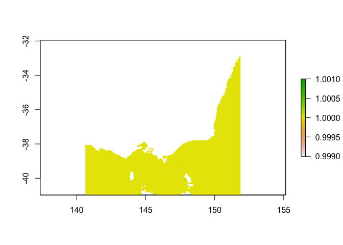
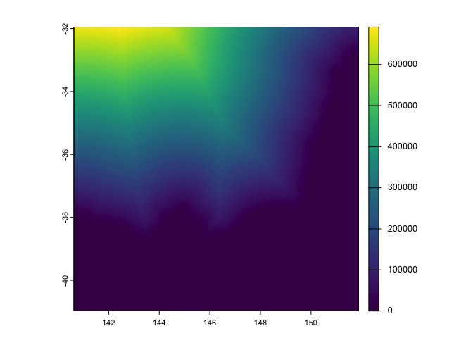
We can do the same thing to figure out distance from the coast:
ras <- vic_elevation %>%
  mask(aus)
values(ras) <- ifelse(is.na(values(ras)), 1, NA)

plot(ras)
dist <- ras %>%
  aggregate(fact = 2) %>%
  rast() %>%
  distance()

plot(dist)
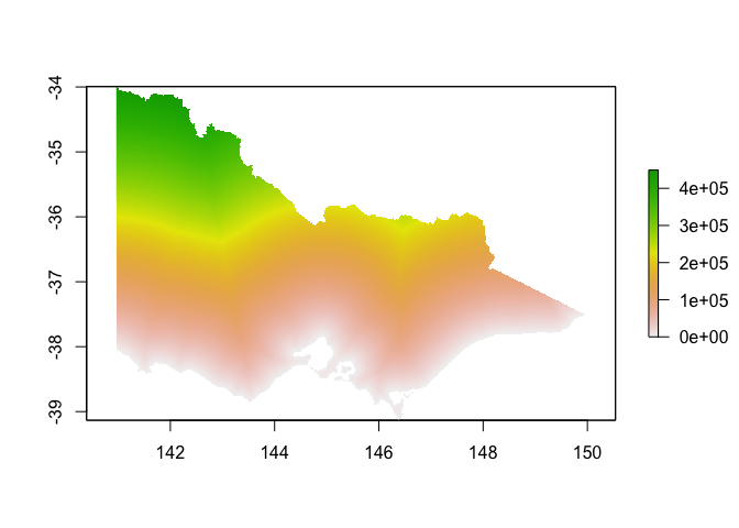
dist_to_coast <- dist %>%
  raster() %>%
  projectRaster(vic_elevation_masked) %>%
  crop(vic_elevation_masked) %>%
  mask(vic_elevation_masked)

plot(dist_to_coast)
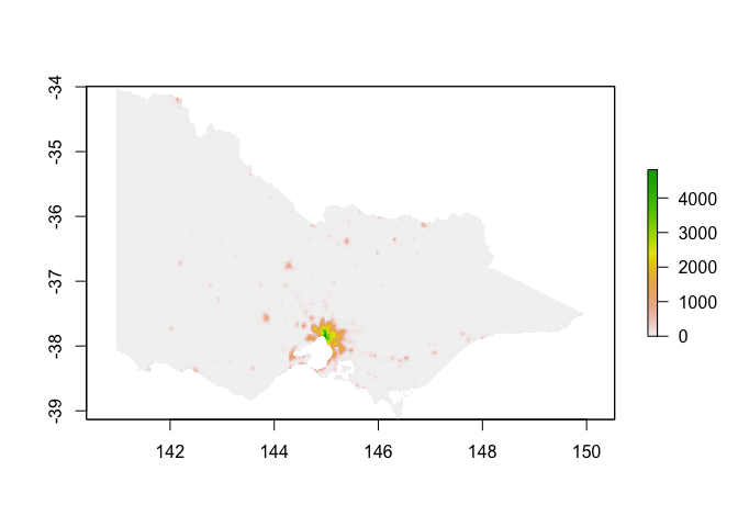
Human population density
Finally let’s grab a raster of human population density for good measure:
library(geodata)
hpop <- population(year = 2020, res = 2.5, path = tempdir())

hpop <- hpop %>%
  raster() %>%
  crop(vic_elevation_buffered) %>%
  projectRaster(vic_elevation_masked) %>%
  mask(vic_elevation_masked)

plot(hpop)
Points: species occurrence
So now we’re raster pros! Let’s grab some point data and compare it to our environmental surfaces …
library(rgbif)
vic_wkt <- vic_buffered %>%
st_simplify(dTolerance = 10000) %>%
st_geometry() %>%
st_as_text()
emus <- occ_search(scientificName = "Dromaius novaehollandiae",
country = "AU",
hasCoordinate = TRUE,
hasGeospatialIssue = FALSE,
geometry = vic_wkt)
emus <- st_as_sf(emus$data,
coords = c("decimalLongitude", "decimalLatitude"),
crs = st_crs(vic))
emus <- filter(emus,
st_intersects(emus, vic, sparse=FALSE)[,1]) # just keep the ones in Victoria
cormorants <- occ_search(scientificName = "Phalacrocorax varius",
country = "AU",
hasCoordinate = TRUE,
hasGeospatialIssue = FALSE,
geometry = vic_wkt)
cormorants <- st_as_sf(cormorants$data,
coords = c("decimalLongitude", "decimalLatitude"),
crs = st_crs(vic))
cormorants <- filter(cormorants,
st_intersects(cormorants, vic, sparse = FALSE)[,1])
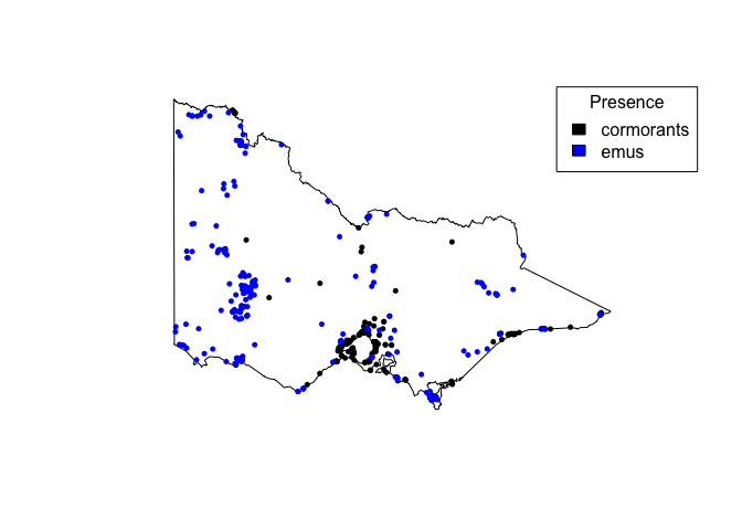
plot(st_geometry(vic))
points(cormorants)
points(emus, col="blue")
legend("topright", fill=c("black", "blue"), c("cormorants", "emus"), title="Presence")
A crap model
All of this to say I’ve been itching for some linear regression!
pseudo_absences <- rasterToPoints(hpop) %>%
data.frame() %>%
mutate(hpop = population_density / sum(population_density))
# There's definitely existing functions to do this ... but now I'm hurrying
# see raster::sampleRandom() ... it doesn't have an option for probs
pseudo_absences_biased <- pseudo_absences[sample(x = 1:nrow(pseudo_absences),
size = nrow(emus),
prob = pseudo_absences$hpop),]
pseudo_absences_random <- pseudo_absences[sample(x = 1:nrow(pseudo_absences),
size = nrow(emus)),]
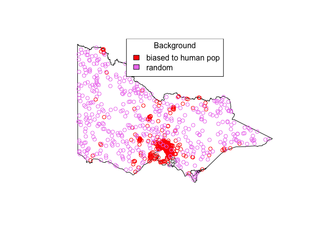
plot(st_geometry(vic))
points(pseudo_absences_biased, col="red")
points(pseudo_absences_random, col="violet")
legend("top", fill=c("red", "violet"), c("biased to human pop", "random"), title="Background")
Let’s fit a model ! (https://rspatial.org/sdm/5_sdm_models.html)
emus_pa <- rbind(emus %>%
st_coordinates() %>%
as.data.frame() %>%
rename(x = X, y = Y) %>%
mutate(pa = 1),
pseudo_absences_biased %>%
dplyr::select(x, y) %>%
mutate(pa = 0))
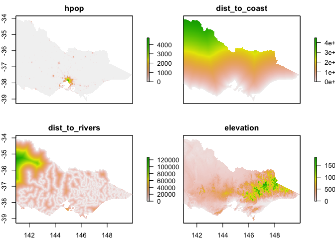
covs_stack <- stack(hpop, dist_to_coast, dist_to_rivers, vic_elevation_masked)
names(covs_stack) <- c("hpop", "dist_to_coast", "dist_to_rivers", "elevation")
plot(covs_stack)
emus_pa <- cbind(emus_pa, raster::extract(covs_stack, emus_pa[,c("x", "y")]))

# Alternatively ...
# emus_pa$population_density <- raster::extract(hpop, emus_pa[,c("x","y")])
# emus_pa$dist_to_coast <- raster::extract(dist_to_coast, emus_pa[,c("x","y")])
# emus_pa$dist_to_rivers <- raster::extract(dist_to_rivers, emus_pa[,c("x","y")])
# emus_pa$elevation <- raster::extract(vic_elevation_masked, emus_pa[,c("x","y")])

m <- glm(pa ~ hpop + dist_to_coast + dist_to_rivers + elevation,
         data = emus_pa,
         family = binomial())

class(m)
## [1] "glm" "lm"
summary(m)
##
## Call:
## glm(formula = pa ~ hpop + dist_to_coast + dist_to_rivers + elevation,
##     family = binomial(), data = emus_pa)
##
## Coefficients:
##                  Estimate Std. Error z value Pr(>|z|)
## (Intercept)     1.269e+00  1.700e-01   7.463 8.46e-14 ***
## hpop           -3.253e-03  3.044e-04 -10.689  < 2e-16 ***
## dist_to_coast  -7.959e-07  8.172e-07  -0.974   0.3301
## dist_to_rivers  2.675e-05  1.290e-05   2.073   0.0382 *
## elevation      -1.343e-03  5.208e-04  -2.579   0.0099 **
## ---
## Signif. codes:  0 '***' 0.001 '**' 0.01 '*' 0.05 '.' 0.1 ' ' 1
##
## (Dispersion parameter for binomial family taken to be 1)
##
##     Null deviance: 1181.10  on 851  degrees of freedom
## Residual deviance:  737.44  on 847  degrees of freedom
##   (4 observations deleted due to missingness)
## AIC: 747.44
##
## Number of Fisher Scoring iterations: 7
m
##
## Call:  glm(formula = pa ~ hpop + dist_to_coast + dist_to_rivers + elevation,
##     family = binomial(), data = emus_pa)
##
## Coefficients:
##    (Intercept)            hpop   dist_to_coast  dist_to_rivers       elevation
##      1.269e+00      -3.253e-03      -7.959e-07       2.675e-05      -1.343e-03
##
## Degrees of Freedom: 851 Total (i.e. Null);  847 Residual
##   (4 observations deleted due to missingness)
## Null Deviance:       1181
## Residual Deviance: 737.4     AIC: 747.4
And make some predictions …
logit_preds <- predict(m, as.data.frame(covs_stack))
prob_preds <- 1 / (1 + exp(-logit_preds))

out <- hpop
values(out) <- prob_preds
Let’s bundle it all into a plot:
vic_rivers <- st_as_sf(rivers)

vic_rivers <- filter(vic_rivers,
                     st_intersects(vic_rivers, vic, sparse = FALSE)[,1])

library(RColorBrewer)
display.brewer.all()
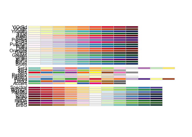
pal <- brewer.pal(9, "Greys")[1:7] %>% # take some of the darker greys out
  colorRampPalette()

library(scales)
##
## Attaching package: 'scales'

## The following object is masked from 'package:purrr':
##
##     discard

## The following object is masked from 'package:readr':
##
##     col_factor

## The following object is masked from 'package:terra':
##
##     rescale
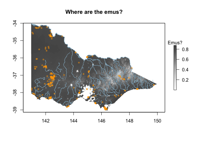
plot(out, main="Where are the emus?", col = pal(100), legend.args=list("Emus?"))
plot(st_geometry(vic_rivers), col='#9ecae1', add=TRUE)
plot(st_geometry(emus), col=alpha("orange", 0.5), add=TRUE, pch=16, cex=0.8)
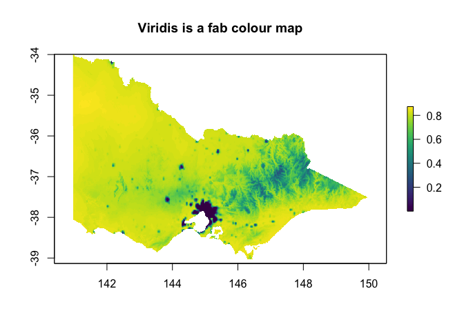
library(viridisLite)
## Warning: package 'viridisLite' was built under R version 4.4.3
?viridis
plot(out, col=viridis(100), main="Viridis is a fab colour map")
There are some reasons why we should doubt this map of where the emus are!
Could you fit a new model using the biased background data? Which of the models is likely more useful?
And here’s some info on where the emus are: https://www.wildlife.vic.gov.au/__data/assets/pdf_file/0025/91384/Emu.pdf
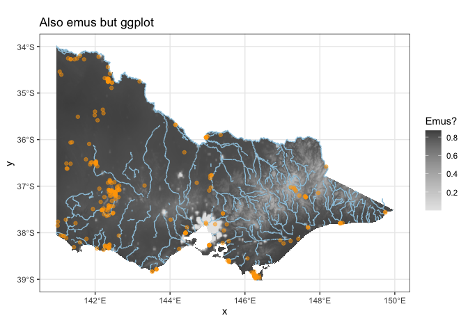
If you would really like to fancy it up, there’s always ggplot:
ggplot(rasterToPoints(out)) +
  geom_raster(aes(x=x, y=y, fill=population_density)) +
  scale_fill_gradientn(colours = rev(grey.colors(100))) +
  geom_sf(data = vic_rivers, aes(geometry=geometry), colour = '#9ecae1') +
  geom_sf(data = emus, colour = "orange", alpha=0.5) +
  labs(title="Also emus but ggplot", fill="Emus?") +
  theme_bw()
Some Rules for mapping (read: Rules for Life)
We’ve all seen a bad map! How did we know it was bad?
- Weird colours are hard to interpret! Try colour brewer (https://colorbrewer2.org/#type=sequential&scheme=BuGn&n=3)
- Colour-blind accessibility! Try colour oracle
(https://colororacle.org) and have a look at what happens to the
base graphics default palette (e.g.,
plot(vic_elevation_masked)) - Dark colours mean more of the thing; red is hot and blue is cold; water should be blue and things that aren’t water shouldn’t be blue; yada yada
- Viridis color maps are often helpful (https://cran.r-project.org/web/packages/viridis/vignettes/intro-to-viridis.html) but don’t overuse !
Conclusion
That’s all for today! We have learned:
- What the types of spatial data are, including points, polygons and rasters
- How to fenangle spatial data, including cropping, masking, trimming and projecting
- How to visualise spatial data in R base graphics (and ggplot)
- How to grab spatial data from a couple of different places, including elevatr and gbif
- How to fit a logistic regression model to presence/background data and make predictions
- Some basic rules for visualising spatial data